Galaxy shRNA-seq Tool Tutorial
The following tutorial illustrates how to use the edgeR shRNA-seq tool on the Galaxy platform.
Prerequisites
To use make use of the instructions in this tutorial you must have access to:- An instance of Galaxy with the shRNAseq tool and all the necessary R packages installed.
- Our shRNAseq Galaxy tool.
Input Data
Three files are required for this tool to function:
- Hairpin Annotation - A tab delimited text file containing the hairpin sequences.
- Sample Annotation - A tab delimited text file containing the sample-specific index sequences and experimental information. AND
- Sequence data - One or more fastq files output by an Illumina sequencer containing the raw sequences from the shRNA-seq screen. OR
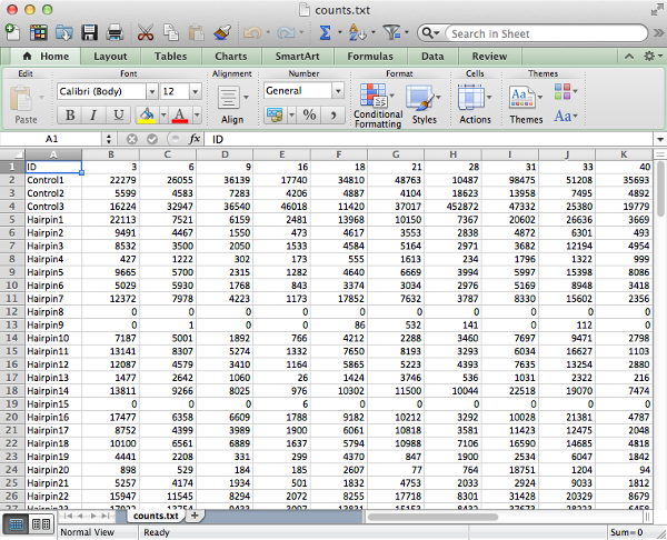
- Counts Table: - Table of counts for each hairpin for each sample.
Both the hairpin and sample annotation data can be entered into any spreadsheet program and saved as tab delimited files:
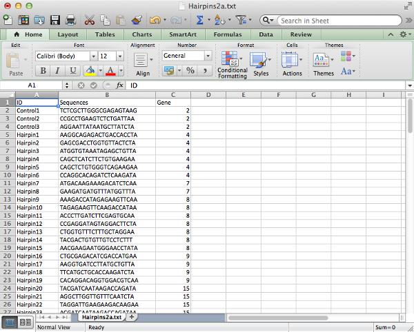
The hairpin annotation table should contain columns:
- ID: Unique identifier for each hairpin.
- Sequences: (if starting from fastq file) The DNA sequence of the hairpin. These must be of uniform length, be unique and correspond to the gene-targeting region (rather than the common sequence).
- Gene: (optional - required for gene-level analysis) The gene on which the hairpin acts.
NOTE: The column names are case-sensitive and should be entered exactly as shown here.
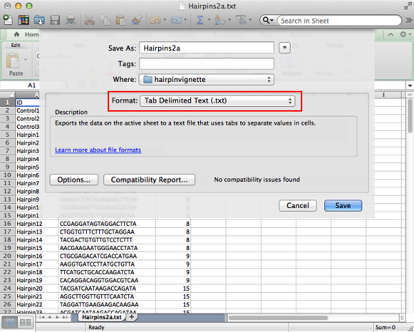
Save the file as tab delimited text to create a text file with table values separated by tab characters.
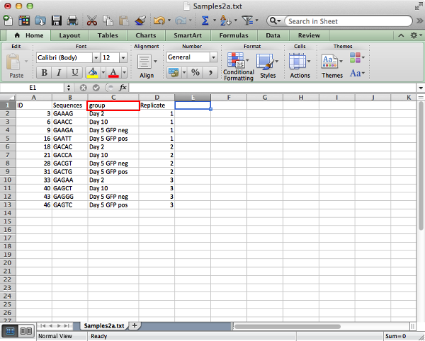
The sample annotation table should contain columns:
- ID: Unique identifier for each sample.
- Sequences: (if starting from fastq file) The DNA index sequence for identifying each sample. These must be of uniform length and be unique.
- group: The experimental group to which the sample belongs. It is important that members of the same group have their group data entered in exactly the same manner with matching case and spacing. Also there must not be any arithmetic operators present as this will create confusion in the contrast equations. (Note the use of pos and neg in place of + and -)
NOTE: Once again the column names are case sensitive and should be entered in exactly as they are shown here. Pay special attention to the 'group' column. Additional columns can be included and will not interfere with the analysis as long as the required columns are present.
If counts have already been calculated then the table of counts can be used as an alternative input in place of fastq files, in this case there should be an ID column that matches exactly the one found in the Hairpin Annotation file and the names of the remaining column should match the ID column of the Sample Annotation file.
Using The Tool
Once the tab delimited files with the necessary information about the experiment have been prepared then the analysis in Galaxy can begin.
It is possible to either upload your data files or access them through shared databases set up by your Galaxy admin. Once uploaded or obtained from a shared database, the files should be available in your history panel to the right.
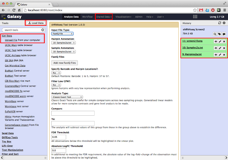
Once the data files are in the history panel they should be input into the tool using the appropriate drop down menus at the top of the tool interface.
To find the tool, type 'shRNA' in the Galaxy search bar (top left) and click on the 'shRNAseq Tool' link
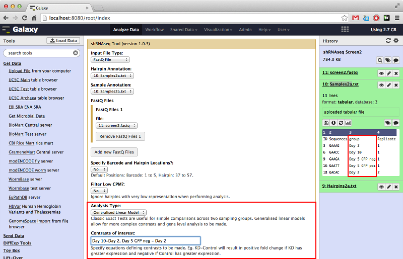
There is the option to perform a classic exact test which allows for simple comparisons between two experimental groups, or a generalized linear model (GLM) analysis which allows for multiple contrasts and gene-level analysis. This tutorial will focus on the latter.
Contrasts are made between experimental groups by inputting equations describing the contrast separated by commas. It is important that the name of the experimental group entered is entered exactly as they are in the sample annotation file. The eye icon in the history panel brings up a convenient display of the data for reminder purposes.
The gene-level analysis option is only available when performing GLM type analysis. It allows us to investigate all hairpins belonging to specific genes as a set to determine if there is any tendencies for all hairpins belonging to a given gene to exhibit positive or negative log-fold-change.
The output will contain a table of genes ranked by ascending p-value for differential representation and selected genes will have barcode plots for visual inspection of the logFC of each hairpin. It is possible to select the genes to produce barcode plots for by either their rank or their unique gene identifier previously specified in the "Gene" column of the sample annotation table.
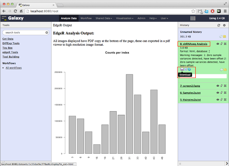
Once the analysis is complete, the results can be viewed by clicking the eye icon in the history panel. This will bring up a page displaying:
- Barplot of the counts per index.
- Barplot of the counts per hairpin (the x-axis will only be labeled if there are 50 or less hairpins).
- MDS plot showing the distance of each sample from each other determined by their leading logFC.
- Smear Plot for each contrast made showing the logFC of each hairpin.
- (Gene Level Analysis only) Barcode plots for the selected genes showing the logFC of hairpins belonging to those genes.
- Table of hairpins in ascending p-value for differential representation for each contrast.
- (Gene Level Analysis only) Table of genes in ascending p-value for differential representation for each contrast.
It's possible to download all the files produced by the tool by clicking the floppy disk icon after expanding the history entry by clicking the name of the entry. This will download a zip archive containing all plots and tables produced by the tool. NOTE: If the download does not start then right-click the icon followed by left-clicking 'Save Link As...'.
Refer to the user guide on hairpin analysis with edgeR for further details on the methods used and how to interpret the various plots and results.
Author
Shian Su (su dot s at wehi dot edu dot au)